Optimisation in the latent space

This post introduces the concept of a latent space and highlights its utility in design problems through an optimisation example. A latent space is a low-dimensional representation of high-dimensional data, where similar items are positioned close together. Recent advances such as variational autoencoders (VAEs) and diffusion models have enabled the learning of very expressive low-dimensional representations of complex design spaces. By shifting optimisation to the latent space, as opposed to optimising the high-dimensional design representation, optimal designs can be identified much more efficiently.

A latent space is an abstract low-dimensional representation of a high-dimensional space…
Items that resemble each other are located close to one another in the latent space
The aim of this post is to demonstrate how the concept of a latent space can be utilised in design problems.
Recent advances such as variational autoencoders (VAEs) and diffusion models have enabled the learning of very expressive low-dimensional representations of complex design spaces.
By shifting optimisation to the latent space, as opposed to optimising the high-dimensional design representation, optimal designs can be identified much more efficiently.
Parametrising the design problem is perhaps the most challenging problem…

mark-hobbs/vae

Motivation

Two major factors that limit our ability to do engineering better are: (1) the computational expense of numerical simulations, and (2) our ability to concisely quantify how different shapes (or designs) are related (our ability to smoothly interpolate between different designs).

Optimisation methods rely on our ability to parameterise the problem but not every design is well-suited to being parametrised. Geometries are typically represented by meshes with thousands to millions of elements.

Imagine if we wanted to find a design that maximises heat dispersion… A simple metric for determining the heat dispersion potential of a given design is the ratio of the surface area to volume. Shapes with a high surface area to volume ratio tend to dissipate or exchange energy with their surrounding more effectively that shapes with a low surface area to volume ratio.

Autoencoders provide a powerful tool for finding low-dimensional representations of high-dimensional data.

By shifting optimisation to the latent space, as opposed to optimising the high-dimensional design representation, optimal designs can be identified much more efficiently.

Latent spaces provide several key advantages in engineering design. They capture the underlying structure and patterns within data, allowing designers to work with meaningful parameters rather than raw features. This enables more intuitive exploration and manipulation of designs, where small changes in the latent space can produce coherent variations in the output.

The mathematical foundation of latent spaces involves dimension reduction techniques that transform complex data into a condensed representation while preserving essential relationships. When properly trained, these models can generate new, valid designs by sampling or navigating through the latent space. Additionally, latent spaces often exhibit interpolation properties, where moving from one point to another creates a smooth transition between corresponding designs.

In optimisation workflows, latent spaces dramatically reduce the search dimensionality. Consider a structural design problem with thousands of potential variables - directly optimising this would be computationally prohibitive. By mapping the problem to a latent space with perhaps just tens of dimensions, optimisation algorithms can operate far more efficiently while still exploring the meaningful variation in the design space.

Dimensionality reduction…

Example problem

The chosen example problem has been selected primarily to enable the promotion of understanding through visual means.

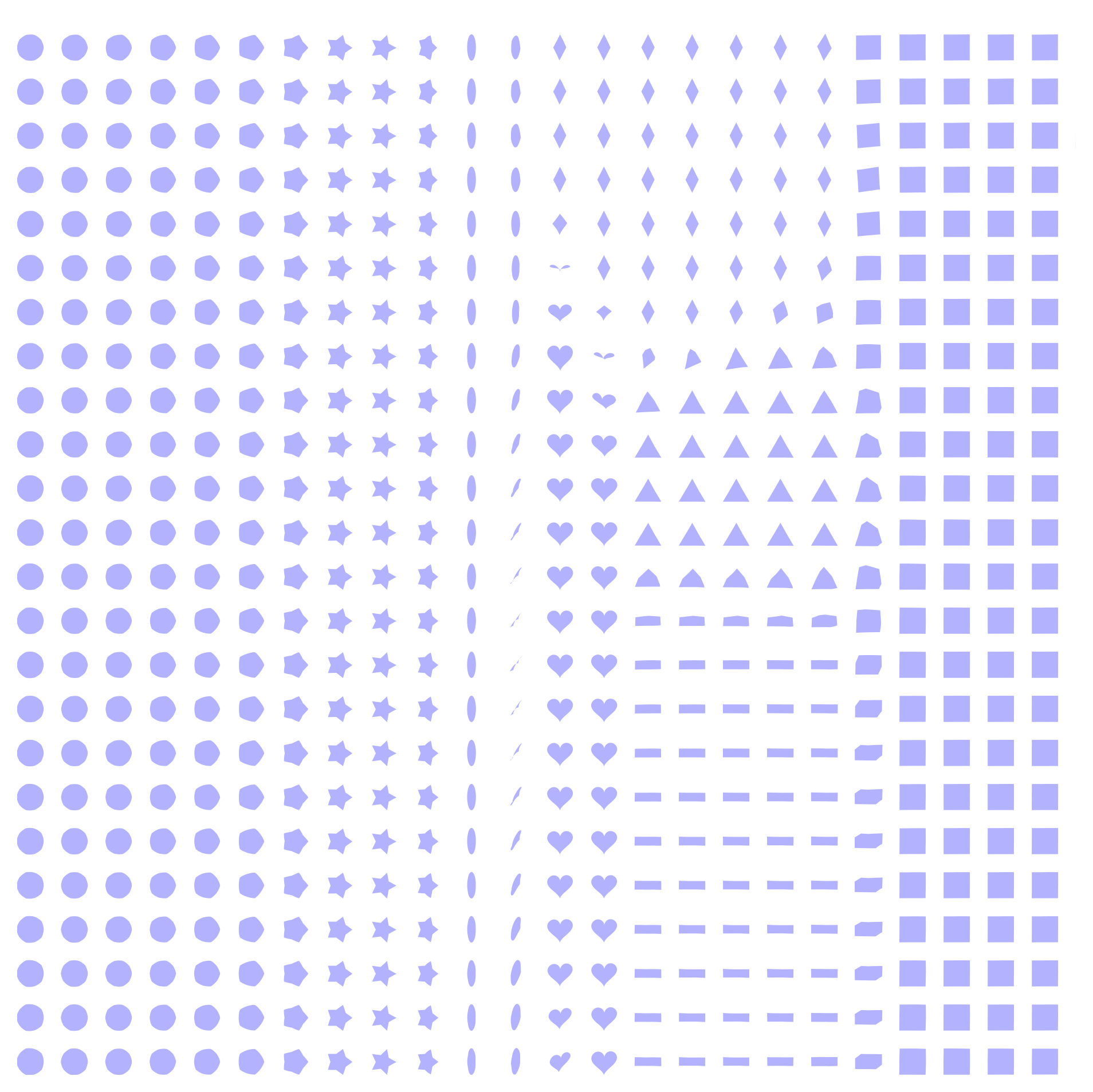
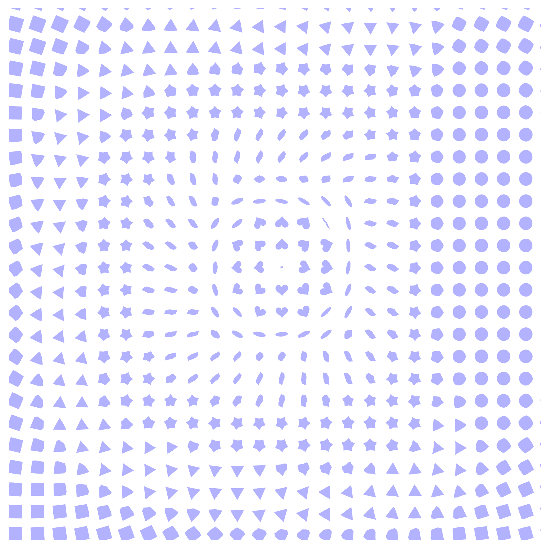
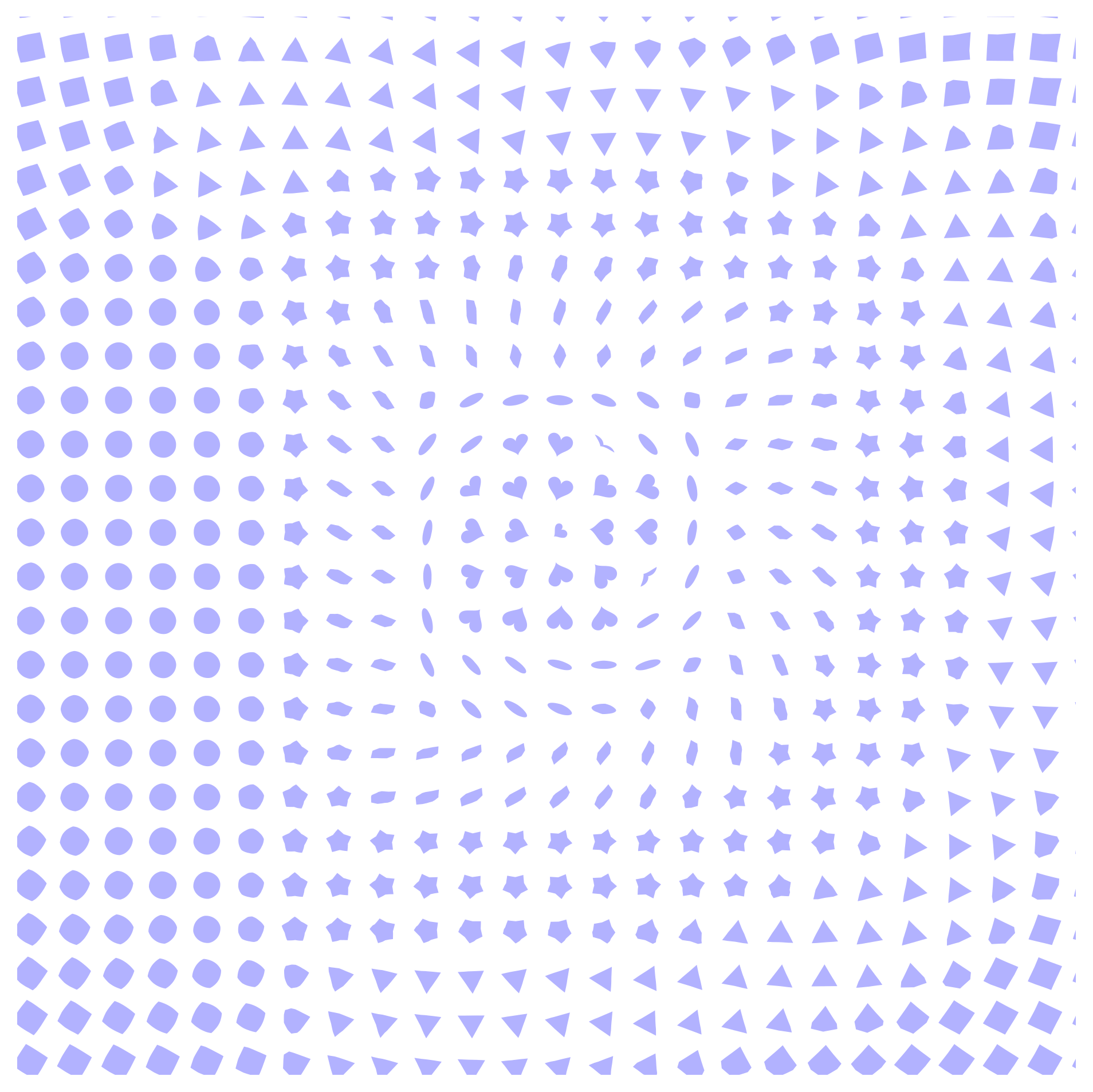
Goal: Train a VAE on a dataset of 2D shapes (e.g., circles, triangles, squares, stars) and use the latent space to interpolate between shapes.

Visualisation: Visualise how shapes smoothly transition and change across the latent space.

Autoencoders

Implementation

Here we outline the implementation using pytorch. We modularise the implementation into three classes:

VAE
Trainer
ShapeData

import torch
import torch.nn as nn


class VAE(nn.Module):
    """
    Variational Autoencoder (VAE) model.

    Parameters
    ----------
    input_dim : int
        Dimension of the input data (degree of freedom)

    latent_dim : int
        Dimension of the latent space.

    Methods
    -------
    encode(x)
        Encodes the input data into mean and log variance of the latent space

    reparameterise(mean, logvar)
        Applies the reparameterisation trick to sample from the latent space

    decode(z)
        Decodes the latent space representation back to the input space

    forward(x)
        Performs a forward pass through the VAE.

    loss_function(reconstructed_x, x, mean, logvar)
        Computes the VAE loss, which is the sum of reconstruction loss and KL divergence
    """

    def __init__(self, input_dim, latent_dim):
        super(VAE, self).__init__()

        self.input_dim = input_dim
        self.latent_dim = latent_dim

        # Encoder
        self.fc1 = nn.Linear(input_dim, 128)
        self.fc2_mean = nn.Linear(128, latent_dim)
        self.fc2_logvar = nn.Linear(128, latent_dim)

        # Decoder
        self.fc3 = nn.Linear(latent_dim, 128)
        self.fc4 = nn.Linear(128, input_dim)

    def encode(self, x):
        h = torch.relu(self.fc1(x))
        mean = self.fc2_mean(h)
        logvar = self.fc2_logvar(h)
        return mean, logvar

    def reparameterise(self, mean, logvar):
        std = torch.exp(0.5 * logvar)
        eps = torch.randn_like(std)
        return mean + eps * std

    def decode(self, z):
        h = torch.relu(self.fc3(z))
        return torch.sigmoid(self.fc4(h))

    def forward(self, x):
        mean, logvar = self.encode(x)
        z = self.reparameterise(mean, logvar)
        reconstructed_x = self.decode(z)
        return reconstructed_x, mean, logvar

    def loss_function(self, reconstructed_x, x, mean, logvar):
        BCE = nn.functional.binary_cross_entropy(reconstructed_x, x, reduction="sum")
        KL_divergence = -0.5 * torch.sum(1 + logvar - mean.pow(2) - logvar.exp())
        return BCE + KL_divergence

import torch.optim as optim
from torch.utils.data import DataLoader


class Trainer:

    def __init__(self, model, dataset, batch_size=32, learning_rate=1e-3, epochs=50):
        self.model = model
        self.dataset = dataset
        self.batch_size = batch_size
        self.learning_rate = learning_rate
        self.epochs = epochs

        self.dataloader = DataLoader(dataset, batch_size=self.batch_size, shuffle=True)
        self.optimiser = optim.Adam(self.model.parameters(), lr=self.learning_rate)

    def train(self):
        for epoch in range(self.epochs):
            self.model.train()
            train_loss = 0
            for batch in self.dataloader:
                self.optimiser.zero_grad()

                reconstructed_batch, mean, logvar = self.model(batch)
                loss = self.model.loss_function(
                    reconstructed_batch, batch, mean, logvar
                )
                loss.backward()
                self.optimiser.step()

                train_loss += loss.item()

            print(
                f"Epoch {epoch+1}/{self.epochs}, Loss: {train_loss / len(self.dataloader)}"
            )

Encoder

Decoder

Discontinuous

def decode(self, z):
    h = torch.relu(self.fc3(z))
    return torch.sigmoid(self.fc4(h))

Continuous

def decode(self, z):
    h = torch.relu(self.fc3(z))
    return self.fc4(h)

Loss function

Loss Term	When to use	Assumes
BCE	Binary or [0,1] normalised inputs	Bernoulli pixels
MSE	Real-valued continuous inputs	Gaussian noise
β-VAE	Need for disentangled representations	Gaussian noise (plus KL control)

Each loss function is a trade-off between accurate reconstruction and learning a smooth well-structured latent space.

def loss_function(self, reconstructed_x, x, mean, logvar):
    """
    Binary Cross-Entropy (BCE) + KL Divergence
    """
    bce = nn.functional.binary_cross_entropy(reconstructed_x, x, reduction="sum")
    kl_divergence = -0.5 * torch.sum(1 + logvar - mean.pow(2) - logvar.exp())
    return bce + kl_divergence

def loss_function(self, reconstructed_x, x, mean, logvar):
    """
    Mean Squared Error (MSE) + KL Divergence
    """
    mse = nn.functional.mse_loss(reconstructed_x, x, reduction="sum")
    kl_divergence = -0.5 * torch.sum(1 + logvar - mean.pow(2) - logvar.exp())
    return mse + kl_divergence

def loss_function(self, reconstructed_x, x, mean, logvar, beta=1.0):
    """
    MSE + β-scaled KL Divergence (β-VAE)
    """
    mse = nn.functional.mse_loss(reconstructed_x, x, reduction="sum")
    kl_divergence = -0.5 * torch.sum(1 + logvar - mean.pow(2) - logvar.exp())
    return mse + beta * kl_divergence

def reconstruction_loss():
    return nn.functional.mse_loss(reconstructed_x, x, reduction="sum")

def similarity_loss():
    return -0.5 * torch.sum(1 + logvar - mean.pow(2) - logvar.exp())

def loss():
    return reconstruction_loss() + similarity_loss()

Visualising the latent space

Each shape is represented by 100 ordered $(x, y)$ coordinate pairs, resulting in a 200-dimensional vector. The objective is to learn a low-dimensional latent space with only 2 dimensions that captures the core geometric features of each shape.