A simple introduction to Bayesian inference

This post introduces Bayesian inference through a simple example that engineers will find familiar, demonstrating the benefits of using probabilistic methods. To maintain accessibility, the use of formal mathematics is minimised. The complete code used to generate all results and figures in this post is available in the following repository: bayesian-inference

Motivation

Model fitting, or calibration, is a crucial aspect of the design process. Engineers rely on numerical models that are calibrated to experimental data before being utilised in downstream design tasks. Once calibrated, these models serve as predictive tools, allowing engineers to simulate the performance of a component or system under varying conditions, optimise design parameters, and make informed decisions in subsequent tasks.

Proper calibration ensures that a model not only fits the data but also accounts for uncertainties inherent in both the data and the model itself, thereby enhancing the reliability and robustness of the design process. This is especially critical when designs operate near performance limits, and small deviations in real-world operating conditions from predicted values can have significant consequences.

Bayesian inference offers a rigorous approach for estimating uncertainty in model parameters, enabling engineers to quantify predictive uncertainties. By quantifying the level of uncertainty, risks associated with overconfidence in model predictions are mitigated, leading to more robust and reliable designs.

Problem statement

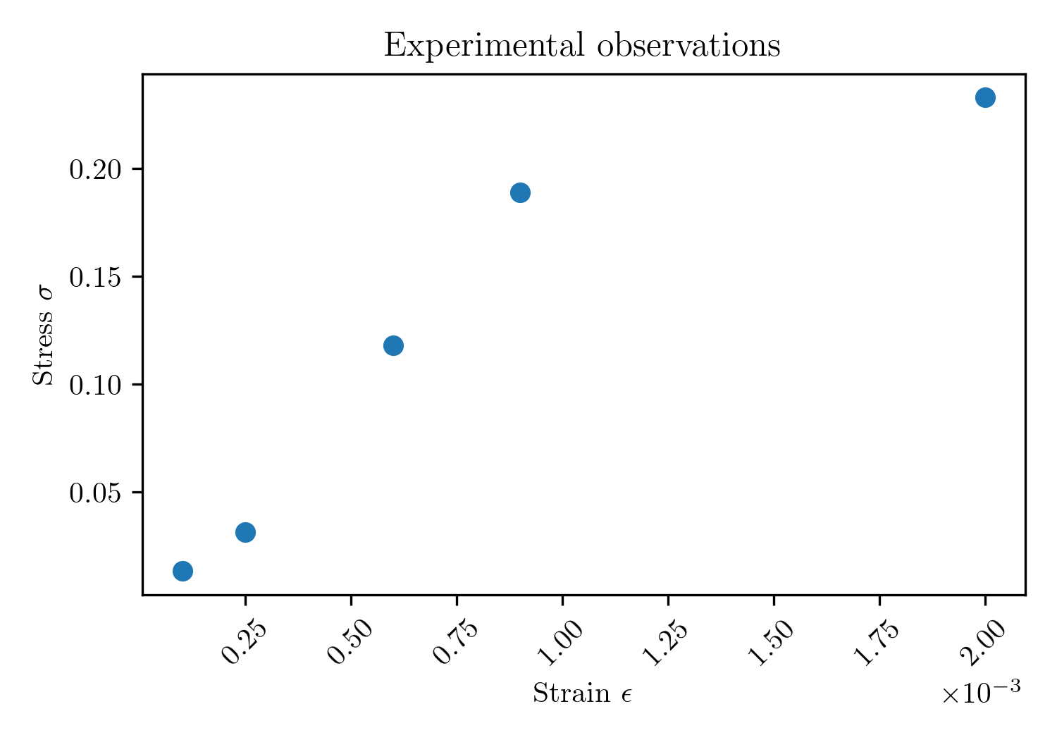
Fit a model to experimental stress-strain ($\sigma$-$\epsilon$) data obtained from a uniaxial tensile test of a material specimen, as depicted in the figure below. The fitted model will inform decision-making and support downstream design tasks. The level of uncertainty in the inferred model parameters should be quantified.

Inverse problems

The problem statement is an example of an inverse problem. The goal of an inverse problem is to estimate an unknown parameter that is not directly observable by using measured data and a mathematical model linking the observed and the unknown.

A mathematical model is selected or designed to describe the relationship between the observed data and the unknown parameter(s), and the model parameters are adjusted to minimise the disparity between the predicted values and actual observations. Iterative optimisation techniques are typically employed to find the best-fitting parameters by minimising a cost function that quantifies the mismatch between the observed data and the predictions of the mathematical model. Through this process of model fitting, predictions or estimations about the unknown parameter(s) can be derived.

Conventional methods have a number of limitations:

1. Overfitting: Conventional methods may overfit the data, particularly when dealing with high-dimensional datasets or when the model is overly complex relative to the available data. Overfitting can result in poor generalisation performance and unreliable estimates of the unknown parameter.

2. Uncertainty quantification: Conventional methods typically do not provide a straightforward means to quantify uncertainty in the estimated parameters. Instead, they offer point estimates that do not capture the inherent uncertainty in the data or the model.

3. Multiple solutions: Inverse problems may have multiple solutions, especially when considering real-world noisy data. This multiplicity of solutions complicates the process of identifying the true underlying parameter, as different sets of parameters may equally well explain the observed data.

4. Ill-posedness: In many cases, inverse problems are ill-posed, meaning that small changes in the observed data can lead to large changes in the estimated parameters. This sensitivity to data perturbations makes it challenging to obtain stable and reliable solutions.

Model $\textbf{f}(\textbf{x})$

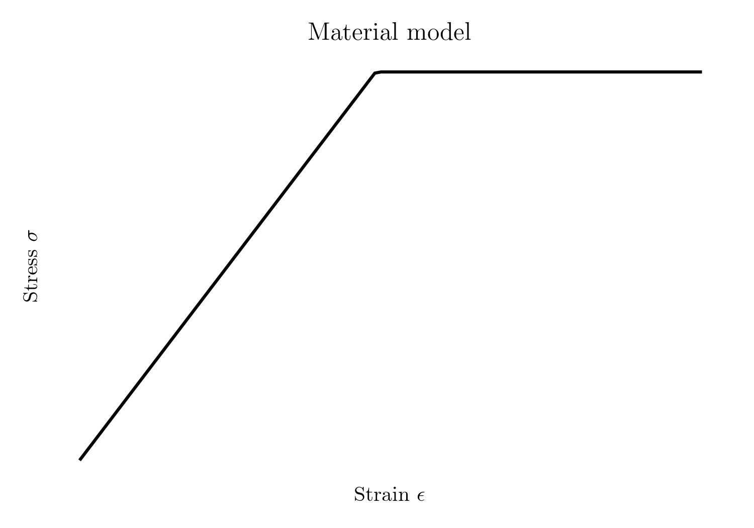
Based on the experimental observations, an expert would likely conclude that the material response is best characterised by a linear elastic-perfectly plastic model. The material model is defined by two parameters: Young’s modulus $E$ and yield stress $\sigma_y$.

The stress-strain relationship for a linear elastic-perfectly plastic material under uniaxial tension can be expressed as:

\[\sigma(\epsilon, \mathbf{x}) = \begin{cases} E\epsilon, & \text{if } \epsilon \leq \sigma_y / E, \\ \sigma_y, & \text{if } \epsilon > \sigma_y / E. \end{cases}\]

where:

• $\sigma$ is the stress,
• $\epsilon$ is the strain,
• $\mathbf{x} = [E, \sigma_y]$ is the vector of model parameters,
• $E$ is Young’s modulus, and
• $\sigma_y$ is the yield stress.

Model fitting

To determine the best-fitting model parameters $\textbf{x}$, the model $\textbf{f}(\textbf{x})$ is fitted to the observed data by minimising the mean squared error (MSE) between the model predictions and the experimental observations. To minimise the error, the model parameters are optimised using techniques such as gradient descent, genetic algorithms and Bayesian optimisation.

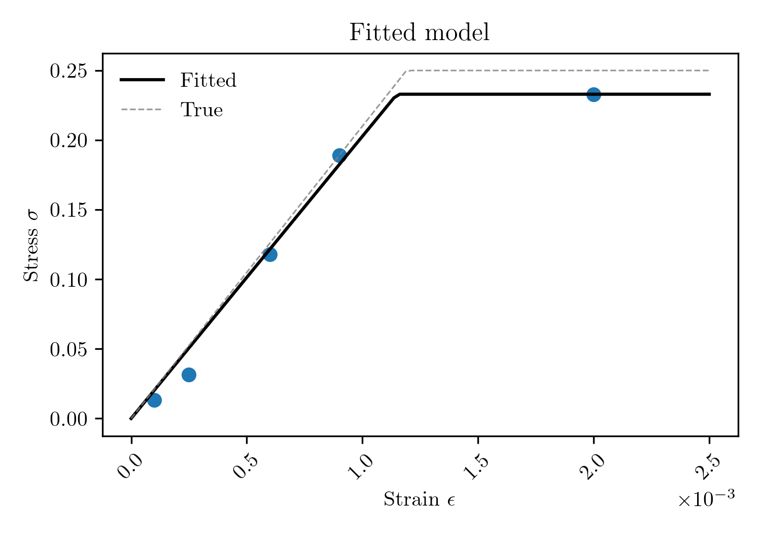
The figure below illustrates the results of this fitting process. The true model, which was used to generate the synthetic observations, is also plotted for reference. Although the disagreement between the true and fitted models may appear small, this fitting process can create a misleading sense of certainty regarding the model parameters. Such overconfidence can have significant consequences for downstream design tasks.

Bayesian inference

A Bayesian framework offers significant advantages for addressing inverse problems. Bayesian inference is the process of updating our beliefs about the probability of an event based on prior knowledge and observed data using Bayes’ theorem. In the context of the presented problem, we update our beliefs about the probability of the parameter values in our model based on prior knowledge and experimental observations. Bayes’ theorem is an extremely powerful concept, particularly in situations where uncertainty exists, data is limited and where prior knowledge or beliefs can be incorporated into the analysis.

Bayes’ Theorem

Bayes’ theorem is used to determine the probability of a hypothesis given observed evidence (the posterior probability). In this example, we can think of the hypothesis and evidence as follows:

• Hypothesis: we hypothesise a model and values for the model parameters, and then we assess how well the model parameters explain the observations
• Evidence: the evidence is in the form of experimental observations (stress-strain data from a uniaxial tensile test)

The posterior probability is a function of the prior probability (prior knowledge) and a ‘likelihood function’ derived from a statistical model for the observed data. Bayesian inference computes the posterior probability according to Bayes’ theorem:

\[\text{Bayes' Theorem:} \quad \pi(\textbf{x}|\textbf{y}) = \frac{\pi(\textbf{x}) \cdot \pi(\textbf{y}|\textbf{x})}{\pi(\textbf{y})}\]

where:

• $\textbf{x}$ denotes a vector with $n_p$ model parameters
• $\textbf{y}$ denotes a vector with $n_m$ observations
• $\pi(\textbf{x})$ is the prior probability (initial beliefs about the parameters)
• $\pi(\textbf{y}|\textbf{x})$ is the likelihood (how well the model parameters explain the data)
• $\pi(\textbf{y})$ is the marginal likelihood or evidence
• $\pi(\textbf{x}|\textbf{y})$ is the posterior probability (updated belief about the model parameters after incorporating the observed data)

Advantages

A Bayesian framework has two core advantages for solving inverse problems:

1. Incorporating prior knowledge: Bayesian inference enables us to incorporate prior knowledge or beliefs about the unknown parameters into the estimation process. This proves particularly useful when dealing with limited data, as it helps regularise the estimation and reduces the risk of overfitting.
2. Uncertainty quantification: Bayesian inference naturally provides a means to quantify uncertainty in the estimated parameters through the posterior distribution. This allows for more informed decision-making by accounting for the inherent uncertainty in the data and the model parameters.

Likelihood $\pi(\textbf{y}|\textbf{x})$

The likelihood function represents the probability of the observed data $\textbf{y}$ given the model parameters $\textbf{x}$. Put another way, the likelihood quantifies the probability that a given set of parameter values produced the observed data. In general, the data-generating process can be modelled as:

\[\textbf{y} = \textbf{f}(\textbf{x}) + \mathbf{\Omega}\]

where $\textbf{f}(\textbf{x})$ denotes the model and is a function of the unknown parameters $\textbf{x}$, and $\mathbf{\Omega}$ represents the noise in the observations. The likelihood is expressed as:

\[\pi(\textbf{y}|\textbf{x}) = \pi_{noise}(\textbf{y} - \textbf{f}(\textbf{x}))\]

The noise model $\pi_{noise}(\mathbf{\Omega})$ captures the distribution of the observational noise $\mathbf{\Omega}$. Noise in the observations arises from imperfections in the measurement apparatus and human error. A Gaussian distribution is a common choice, modelling noise as normally distributed with a mean of zero and a specified variance, although more complex distributions may be necessary for certain datasets.

Prior $\pi(\textbf{x})$

The prior represents our initial beliefs about the model parameters before observing any data. It allows us to incorporate knowledge from prior studies and expert opinions about the the probable values of the parameters. For the model parameters $\textbf{x}$, the prior can take different forms, but unless there is evidence to suggest otherwise, a normal distribution is commonly used:

\[\pi(\textbf{x}) \propto \exp\left(-\frac{(\textbf{x} - \overline{\textbf{x}})^2}{2\sigma^2_{\textbf{x}}}\right)\]

This expresses the belief that the parameters $\textbf{x}$ are normally distributed around a mean $\overline{\textbf{x}}$ with a standard deviation $\sigma_{\textbf{x}}$.

Posterior $\pi(\textbf{x}|\textbf{y})$

The posterior represents our belief about the parameters $\textbf{x}$ after observing the data $\textbf{y}$. The posterior is given by:

\[\pi(\textbf{x}|\textbf{y}) \propto \pi(\textbf{x}) \cdot \pi(\textbf{y}|\textbf{x})\]

In this form, the posterior incorporates both the prior belief about the parameters and the likelihood of the observed data given those parameters. After normalising, we get the updated distribution for the parameters:

\[\pi(\textbf{x}|\textbf{y}) = \frac{1}{C} \pi(\textbf{x}) \cdot \pi(\textbf{y}|\textbf{x})\]

where $C$ is a normalisation constant ensuring that the integral of the posterior over $\textbf{x}$ equals 1. In most cases, this constant can be ignored, as the primary interest lies in the relative probabilities of different parameter candidates, and the unnormalised posterior provides all the necessary information.

Approximating the posterior

The posterior can only be determined analytically in a limited number of simple cases where the prior and likelihood are conjugate and a closed-form solution can be derived. For more complex real-world problems, numerical methods are used to approximate the posterior distribution; however, this is a non-trivial task when the parameter space is high-dimensional or the model is computationally expensive to evaluate.

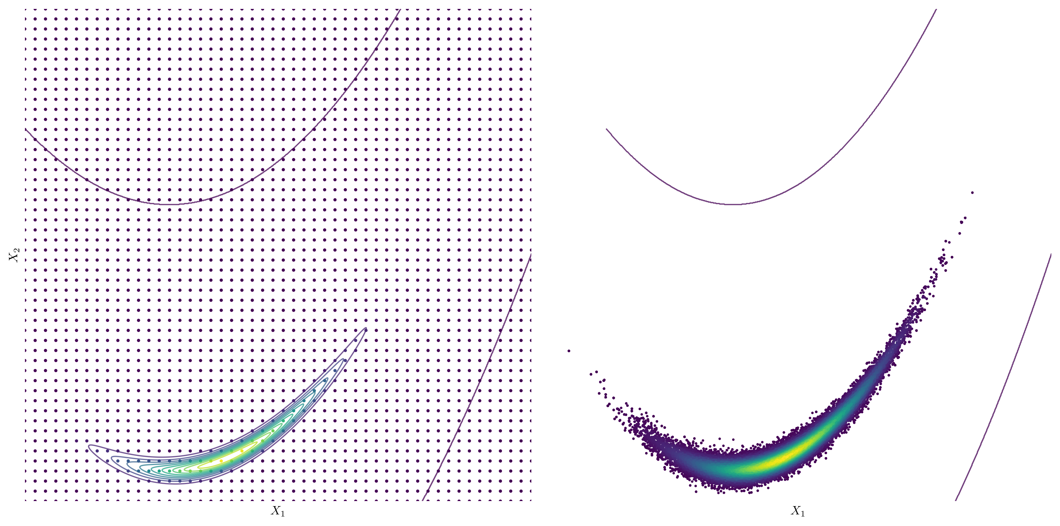
Grid Search

In cases where analytical solutions are infeasible due to complex or non-standard distributions, grid search offers a practical numerical approach. The parameter space is discretised into a grid, and the posterior probability is computed at each grid point, providing an estimate of the posterior distribution. While grid search is straightforward to implement, it suffers from the curse of dimensionality, where the number of required evaluations grows exponentially with the number of dimensions. If the model $\textbf{f}(\textbf{x})$ is computationally expensive, for example, a numerical simulation, grid search is often impracticable. Additionally, many evaluations are effectively ‘wasted’ in regions where the posterior density is low. This inefficiency underscores the need for more advanced methods that concentrate the search on regions of interest — specifically, areas where the posterior density is high.

Markov Chain Monte Carlo (MCMC)

When the search space becomes larger, or the model is expensive to evaluate, it can become infeasible to do an exhaustive search and we must turn to randomised searches. Markov Chain Monte Carlo (MCMC) methods are the most common approach in such scenarios. The aim of MCMC is to randomly walk through the parameter space, while the fraction of time spent at each state $\theta_i$ is $\propto$ the unormalised posterior.

MCMC methods offer a powerful and versatile approach to estimate the posterior distribution, particularly in high-dimensional and complex models where analytical solutions or grid search are impractical. MCMC algorithms, such as Metropolis-Hastings and Gibbs sampling, generate a Markov chain that asymptotically converges to samples from the target posterior distribution. These methods iteratively propose candidate parameter values, accepting or rejecting them based on a defined acceptance criterion that preserves the desired distribution. MCMC provides flexibility in handling complex models and can efficiently explore the parameter space, even in cases of high dimensionality or non-standard distributions. Advanced techniques, such as Hamiltonian Monte Carlo, further improve the accuracy and efficiency of Bayesian inference by leveraging gradient information to enhance the exploration of the parameter space.

Summary

Each of these methods has its strengths and limitations, and the choice depends on factors such as the computational expense of the model $\textbf{f}(\textbf{x})$, computational resources available and the desired accuracy of the posterior estimation. For a visual guide to design space exploration and its connection to MCMC and grid search, refer to this post.

Posterior Analysis

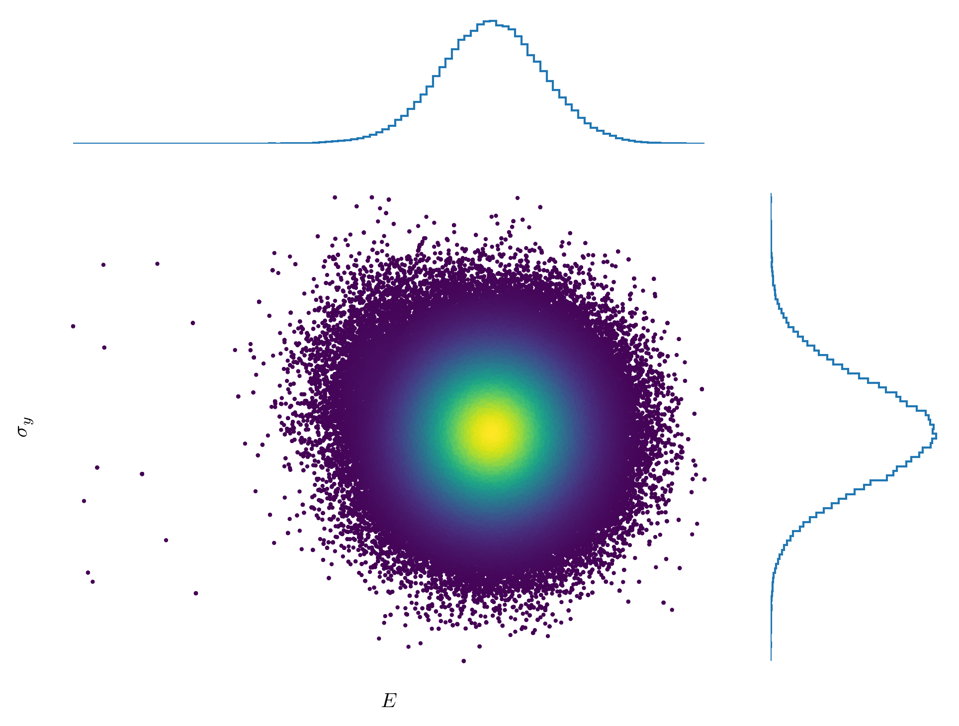
To efficiently obtain an accurate prediction of the posterior distribution, we typically employ MCMC methods. In this post, we have utilised an Adaptive Metropolis-Hastings sampler to approximate the posterior distribution. The process of tuning MCMC samplers and ensuring that they have adequately explored the posterior and achieved convergence is beyond the scope of this post. However, it is a crucial aspect of reliable Bayesian inference, as poor tuning or insufficient exploration can lead to biased estimates or inaccurate conclusions. The figure below illustrates a well-sampled posterior with good coverage of the parameter space.

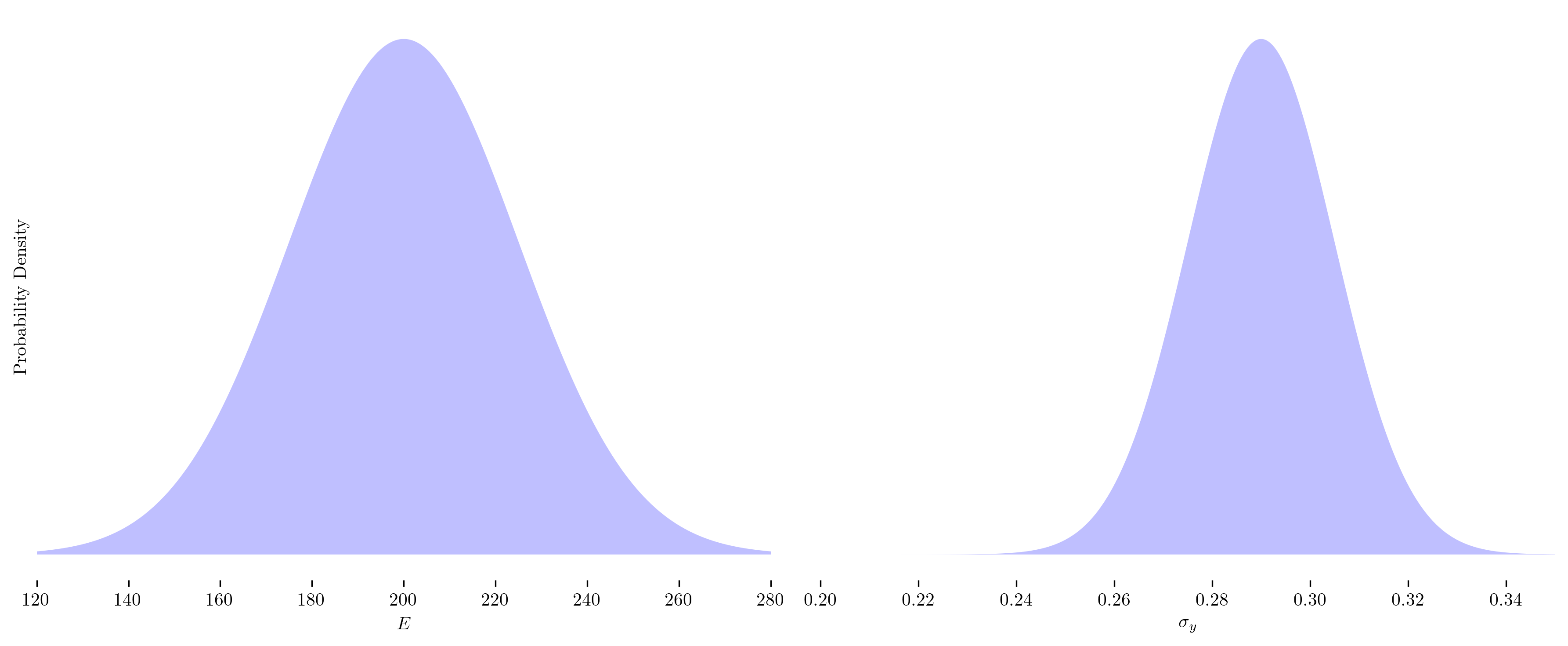
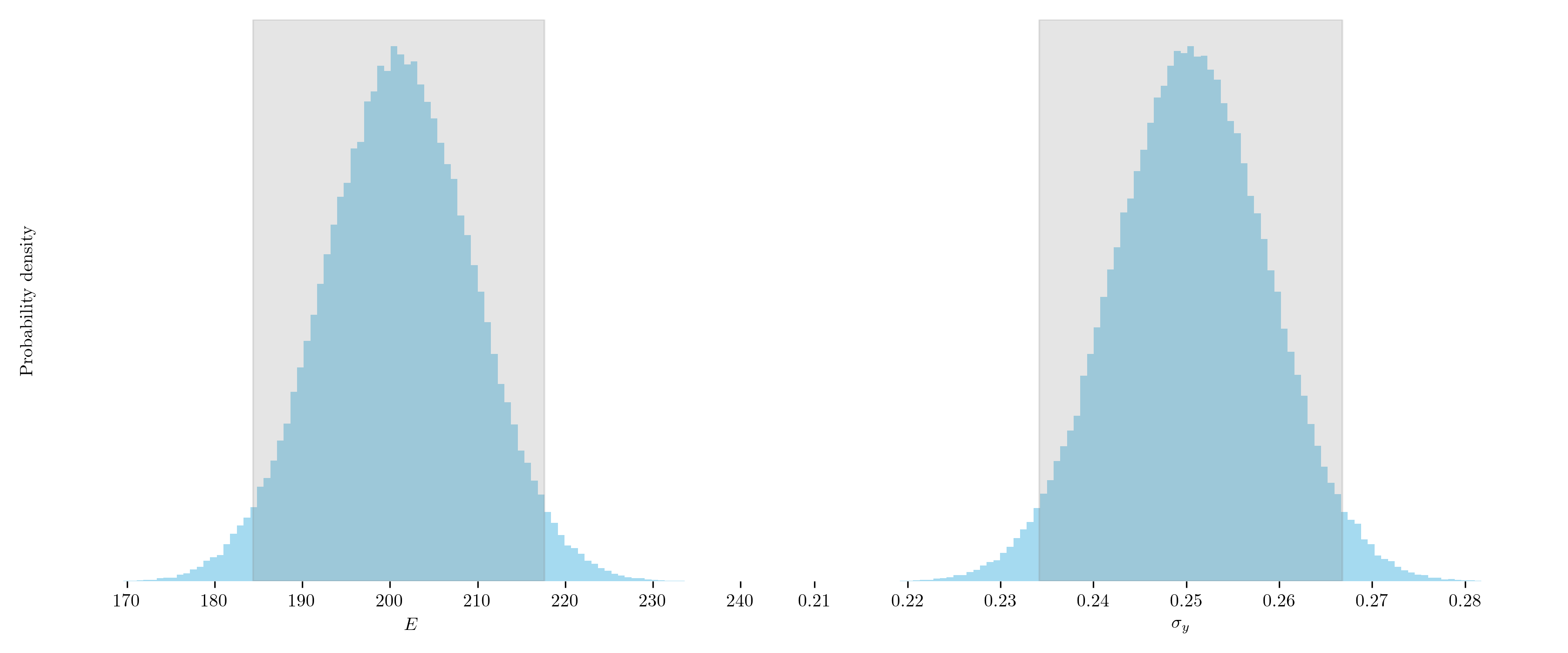
Once the posterior distribution has been sampled, the next step is to analyse it to extract statistical summaries, draw meaningful conclusions and make informed predictions. This analysis often includes estimating quantities such as means, variances and credible intervals, as well as visualising the results to better understand the underlying uncertainty and parameter correlations. The below figure illustrates our belief about the individual model parameters, with the shaded region representing the 95% credible interval.

Posterior Predictive Distribution

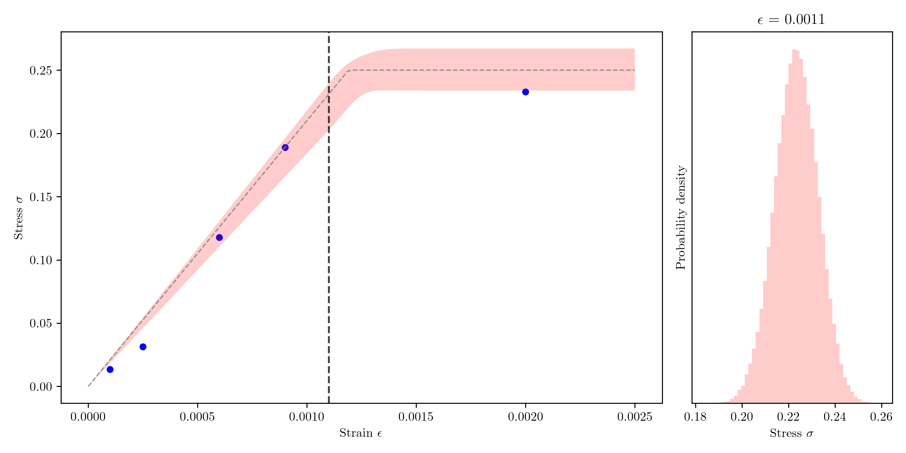
The posterior distribution represents our belief about the model parameters given the observed data. By utilising this information in downstream design tasks, it is possible to quantify the uncertainty in our simulations and models, thereby enhancing design robustness.

By propagating the uncertainty in the model parameters forward through the model, we gain insight into the uncertainty in our predictions. For example, if the objective is to determine the stress in a component at a specific strain value, a standard approach would return a single deterministic estimate. In contrast, a probabilistic approach provides a distribution of the stress, offering a much deeper understanding of the range of potential outcomes.

Why are density values omitted?

Probability density values are omitted from posterior plots to emphasise the shape of the distribution, focussing attention on high-probability regions and the relative likelihood of parameter values. Absolute density values offer little interpretive value, as posterior densities are often normalised and primarily used for comparison.

Conclusion

Given experimental data from a uniaxial tensile test of a material specimen, we hypothesised that the material response could be described by a linear elastic-perfectly plastic material model. To determine the model parameters, we initially employed conventional optimisation techniques to minimise an error function quantifying the discrepancy between the observed data and the model predictions. However, this approach yields point estimates of the parameters, which can create a false sense of certainty and potentially lead to significant consequences in downstream design tasks.

To address this issue, we employed a Bayesian framework to infer the parameters in the material model, while accounting for noise in the experimental observations. Bayesian inference provides an estimate of the posterior distribution of the model parameters rather than deterministic point estimates. Learning comes from two sources: (1) the evidence provided by the observed data and (2) prior knowledge about the likely values of the model parameters.

We approximated the posterior using an Adaptive Metropolis-Hastings sampler and demonstrated how this information can be applied to downstream design tasks to quantify uncertainty in predictions (e.g., numerical simulations). A Bayesian approach provides a rigorous framework for designing under uncertainty, offering a deeper understanding of the uncertainty in our predictions and safeguarding against overconfidence.

Finally, it is important to remember that when fitting a model to data, errors exist in both the data and the model. In the presented example, we have only accounted for errors in the data, while neglecting potential inaccuracies in the model itself.